In our previous article on onchain data indexing, we covered how to fetch and stream onchain data efficiently, which is only half the equation. To illustrate ClickHouse's capabilities for storing and querying onchain data at scale, we ran an experiment on the Tempo testnet (moderato) chain indexing data from genesis, which produced about 3.5 billion rows and 800 GB of uncompressed data across blocks, transactions, and logs.
All benchmarks in this article were run on a Kubernetes cluster of 3 nodes (8 vCPU, 32 GB RAM each) running a replicated ClickHouse setup, with each ClickHouse instance allocated 4 vCPU and 16 GB RAM.
Ingestion
The performance gains from streaming onchain data for indexing are only meaningful if the underlying storage layer can ingest data at roughly the same rate it is being produced. This is an area where ClickHouse shines. It can consume millions of rows per second, provided a few best practices are followed to leverage its full capabilities. There are two main levers that have a significant impact on ClickHouse ingestion speed:
-
Data format: The recommended format is
Nativebecause it is the fastest and has the best compression ratios across codecs (see ClickHouse input format benchmarks). Unfortunately, at the time of writing, the Rust ClickHouse client only supportsRowBinary(although there are plans to supportNative) which is still fast enough. -
Batching: ClickHouse supports both client-side and server-side batching. The main reason for batching is that ClickHouse processes and stores data in "parts", so sending individual rows or small batches results in a lot of small parts, which creates CPU overhead during merges. The recommended batch size is around 10K to 100K rows per batch.
With these two levers, we were able to ingest the full Tempo testnet chain (3.5 billion rows) in roughly 3.5 hours, or about 270K rows per second. Below are a few screenshots of memory, CPU, IOPS, and throughput during ingestion.
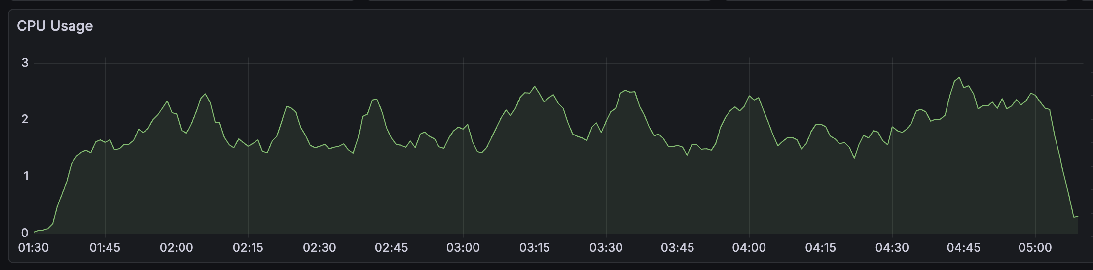
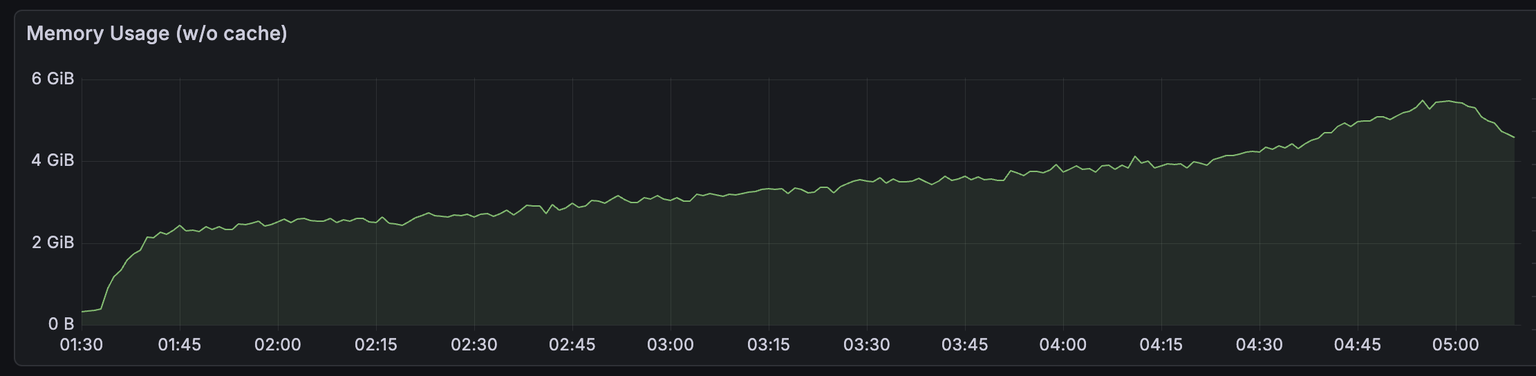
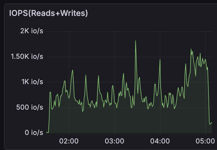
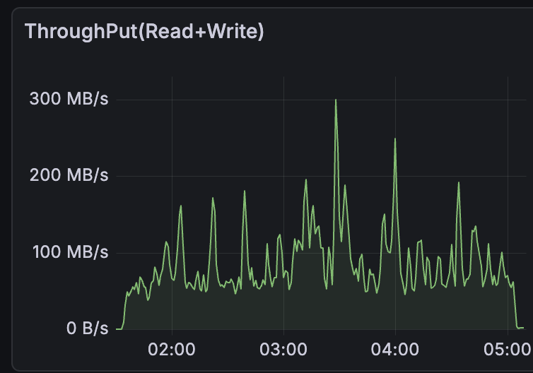
A few things stand out from these charts. CPU stays flat at around 1.5 to 2 cores for the entire run, showing that ingestion at this scale is not CPU-bound. Memory grows steadily from 0 to about 5 GiB rather than spiking, which reflects ClickHouse flushing parts to disk incrementally as batches arrive. The IOPS and throughput charts show periodic spikes, up to ~1.8K io/s and ~300 MB/s, caused by background merge operations where ClickHouse consolidates smaller parts into larger ones, which is typical of write-heavy ClickHouse workloads. These spikes only become problematic if the storage layer cannot absorb them fast enough, resulting in part explosion or ingest lag.
Schema
The next bottleneck after ingestion is how we represent data at the storage layer. A proper schema definition can make a night and day difference in query and storage efficiency in ClickHouse. The most important things to look out for in a table schema are the ORDER BY and PRIMARY KEY clauses. This is because, in MergeTree family tables, the ORDER BY clause, also known as the sorting key, determines how data is physically sorted on disk. Using the correct sort keys can enable huge performance gains as it allows for data skipping.
Consider the following logs table definition:
CREATE TABLE IF NOT EXISTS logs
(
    block_number UInt64,
    block_timestamp UInt64,
    transaction_hash FixedString(32),
    transaction_index UInt64,
    log_index UInt64,
    address FixedString(20),
    topics Array(FixedString(32)),
    data String,
    is_deleted UInt8 DEFAULT 0,
    _version DateTime64(3) DEFAULT now64()
)
ENGINE = ReplacingMergeTree(_version, is_deleted)
ORDER BY (address, topics[1], data)
PRIMARY KEY (address);
While it is tempting to sort by address and topics[1] (ClickHouse arrays are 1-indexed) since most queries filter on both, this trades storage efficiency for query performance. High-cardinality columns like address compress poorly because adjacent rows on disk rarely share the same value, giving the codec little to work with. A better sorting key would be (block_number, transaction_index, log_index) because they are sequential integers that compress very well. We can then use a materialized view with address as the sort key for better query performance, which we will cover later in this article. The main rule of thumb for the primary table sorting key is to use low-cardinality columns first, then columns that are frequently used in WHERE queries.
Another storage choice worth calling out is using FixedString for fixed-length byte fields rather than their hex string representations. A transaction hash stored as FixedString(32) takes 32 bytes, whereas the equivalent hex string (VARCHAR(66) including the 0x prefix) takes 66 bytes (more than twice the space). The same applies to addresses (FixedString(20) vs 42-byte hex) and topics (FixedString(32)). Across billions of rows this difference is substantial, and FixedString values also compress better since they avoid the character overhead of ASCII hex encoding.
We can further improve storage by adding compression codecs to the schema definition. The ClickHouse documentation recommends ZSTD as it offers the best compression ratios. We also use Delta in combination with ZSTD to improve compression of dates and integer sequences. So the optimal logs table looks like this:
CREATE TABLE IF NOT EXISTS logs
(
    block_number UInt64 CODEC(Delta, ZSTD),
    block_timestamp UInt64 CODEC(Delta, ZSTD),
    transaction_hash FixedString(32) CODEC(ZSTD),
    transaction_index UInt64 CODEC(Delta, ZSTD),
    log_index UInt64 CODEC(Delta, ZSTD),
    address FixedString(20) CODEC(ZSTD),
    topics Array(FixedString(32)) CODEC(ZSTD),
    data String CODEC(ZSTD(3)),
    is_deleted UInt8 DEFAULT 0,
    _version DateTime64(3) DEFAULT now64()
)
ENGINE = ReplacingMergeTree(_version, is_deleted)
ORDER BY (block_number, transaction_index, log_index)
PRIMARY KEY (block_number, transaction_index, log_index);
Across the full Tempo testnet chain data, these choices bring the total on disk footprint down to ~93 GiB from ~800 GiB of uncompressed data (an overall 8.6x compression ratio). logs benefit the most due to high repetition in addresses and topics across rows, while blocks compress the least since most fields are unique per row.
| Table | Uncompressed | Compressed | Ratio |
|---|---|---|---|
| logs | 458.65 GiB | 32.99 GiB | 13.9x |
| txs | 339.90 GiB | 58.54 GiB | 5.81x |
| blocks | 1.99 GiB | 1.26 GiB | 1.57x |
| total | ~800 GiB | ~93 GiB | ~8.6x |
Breaking it down by column for the logs table shows where the codec choices pay off:
| Column | Uncompressed | Compressed | Ratio |
|---|---|---|---|
| topics | 226.61 GiB | 23.11 GiB | 9.81x |
| data | 97.63 GiB | 6.24 GiB | 15.64x |
| address | 44.80 GiB | 2.48 GiB | 18.06x |
| transaction_index | 17.92 GiB | 617.52 MiB | 29.72x |
| log_index | 17.92 GiB | 381.40 MiB | 48.11x |
| block_number | 17.92 GiB | 54.70 MiB | 335.46x |
| block_timestamp | 17.92 GiB | 47.76 MiB | 384.22x |
The Delta + ZSTD codec on sequential integers is extremely effective as block_number and block_timestamp compress at over 300x, making them nearly free on disk. The bulk of the storage footprint comes from topics, data, and address, which have high entropy and can only be compressed with ZSTD alone. This also illustrates why using address or topics[1] as a sort key hurts compression: those columns don't benefit from delta encoding and their high cardinality means adjacent rows on disk have dissimilar values, leaving little for ZSTD to exploit.
Reorg handling
Despite its incredible performance, ClickHouse doesn't do well with frequently updated data. However, our use case requires us to handle reorgs, which means deleting multiple rows occasionally. For such use cases, it is recommended to use specialized table engines that offer eventual consistency by handling updates at merge time. In the logs schema above, we used the ReplacingMergeTree engine. This allows us to specify a version and deleted column, which are used by the engine to deduplicate rows by picking the row with the highest version and removing rows that are deleted. This means that reorgs are handled by inserting new rows with is_deleted = 1 and _version = now().
The downside of this approach is that SELECT queries can return inaccurate data between merges. ClickHouse offers the FINAL keyword, which can be used to force a merge at query time, although with a performance penalty. We can also filter by is_deleted = 0 in our queries without performance loss, given that we are only deleting rows and not updating them.
Querying data
In some cases, although the choice of sorting key provides great storage performance, it can result in poor query performance. To illustrate this, let's use the logs table defined above to list the 10 most recently minted TIP-20 tokens. TIP-20 is Tempo's standard for stablecoins, similar to ERC-20 on Ethereum. For the purpose of this example, the main thing to know is that TIP-20 tokens are created using a factory contract whose address is 0x20Fc000000000000000000000000000000000000. To fetch newly created TIP-20 tokens, we need to filter recent logs by the contract address and the topic selector for the TokenCreated event, which is keccak256("TokenCreated(address,string,string,string,address,address,bytes32)") or 0x44f7b8011db3e3647a530b4ff635726de5fafc8fa8ad10f0f31c0eb9dd52fc65. The query looks like this:
SELECT
    block_number,
    lower(hex(address)) AS address_hex,
    lower(hex(topics[1])) AS topic0_hex,
    data
FROM logs
WHERE
    address = unhex('20Fc000000000000000000000000000000000000')
    AND topics[1] = unhex('44f7b8011db3e3647a530b4ff635726de5fafc8fa8ad10f0f31c0eb9dd52fc65')
    AND is_deleted = 0
ORDER BY block_number DESC
LIMIT 10;
Running this against the full Tempo testnet chain, the cold and warm query stats are:
| Metric | Cold | Warm |
|---|---|---|
| Duration | 112 ms | 11 ms |
| Rows read | 31,504 | 31,504 |
| Bytes read (compressed) | ~4.63 MiB | ~332 KiB |
| Memory usage | ~1013 KiB | ~1012 KiB |
| CPU | 120,820 µs | 17,227 µs |
Normally, a predicate that doesn't align with the sort key forces ClickHouse to scan every granule, and the query plan confirms this: Granules: 293608/293608, meaning ClickHouse cannot skip on address or topics[1] at all because the table is ordered by (block_number, transaction_index, log_index). Yet only 31,504 rows are read out of 3.5 billion, because with ORDER BY block_number DESC LIMIT 10, ClickHouse scans from the newest end of the table and stops as soon as it has 10 matching rows. We can stress the current layout by searching for a non-existent topic selector:
SELECT
    block_number,
    lower(hex(address)) AS address_hex,
    lower(hex(topics[1])) AS topic0_hex,
    data
FROM logs
WHERE
    address = unhex('20Fc000000000000000000000000000000000000')
    AND topics[1] = unhex('ffffffffffffffffffffffffffffffffffffffffffffffffffffffffffffffff')
    AND is_deleted = 0
ORDER BY block_number DESC
LIMIT 10;
This query is pathological for the base table because there are no matches to stop on early, so the engine has to keep walking the main table while still being unable to prune on address or topics[1].
To improve the performance of this type of query, we can add a new table and a backing incremental materialized view with a different sorting key. ClickHouse incremental materialized views let us maintain a derived table that is updated every time rows are inserted into the primary table. This shifts work from query time to insert time.
  CREATE TABLE IF NOT EXISTS logs_by_topic0
  (
      topic0 FixedString(32) CODEC(ZSTD),
      block_number UInt64 CODEC(Delta, ZSTD),
      transaction_index UInt64 CODEC(Delta, ZSTD),
      log_index UInt64 CODEC(Delta, ZSTD),
      address FixedString(20) CODEC(ZSTD),
      is_deleted UInt8 DEFAULT 0,
      _version DateTime64(3) DEFAULT now64()
  )
  ENGINE = ReplacingMergeTree(_version, is_deleted)
  ORDER BY (address, topic0, block_number, transaction_index, log_index);

  CREATE MATERIALIZED VIEW IF NOT EXISTS mv_logs_by_topic0
  TO logs_by_topic0
  AS
  SELECT
      topics[1] AS topic0,
      block_number,
      transaction_index,
      log_index,
      address,
      is_deleted,
      _version
  FROM logs
  WHERE length(topics) >= 1;
With the new materialized view, the non-existent topic query becomes:
SELECT
    l.block_number,
    lower(hex(l.address)) AS address_hex,
    lower(hex(l.topics[1])) AS topic0_hex,
    l.data
FROM logs AS l
WHERE (l.block_number, l.transaction_index, l.log_index) IN
(
    SELECT
        block_number,
        transaction_index,
        log_index
    FROM logs_by_topic0 AS t
    WHERE
        t.address = unhex('20Fc000000000000000000000000000000000000')
        AND t.topic0 = unhex('ffffffffffffffffffffffffffffffffffffffffffffffffffffffffffffffff')
        AND t.is_deleted = 0
)
AND l.is_deleted = 0
ORDER BY l.block_number DESC
LIMIT 10;
The subquery is necessary because logs_by_topic0 only stores a subset of columns, enough to find matching rows while keeping the table's footprint small. The query works in two steps: the subquery uses the materialized view's sort key (address, topic0, block_number, ...) to skip directly to the matching granules and return the row coordinates (block_number, transaction_index, log_index), the outer query then uses those coordinates to do point lookups against logs, which is efficient because (block_number, transaction_index, log_index) is the primary key of the main table.
A JOIN is more expensive here because ClickHouse has to scan and stream rows from both tables simultaneously, whereas the IN subquery lets it fully resolve the matching coordinates first and then perform targeted primary-key lookups. For the non-existent topic case, the IN pattern is dramatically faster than the equivalent JOIN. Measured on the same cluster, the IN query took 7 ms, read 0 rows, and used only 16.86 KiB of memory because ClickHouse resolved the subquery first, realized it produced an empty set, and pruned the main table entirely. The equivalent JOIN took 79 ms, read 65,536 rows, touched all 293,608 marks of the base table, and used about 10 MiB of memory.
| Query shape | Duration | Rows read | Compressed bytes read | Memory |
|---|---|---|---|---|
IN subquery | 7 ms | 0 | 0 B | 16.86 KiB |
JOIN | 79 ms | 65,536 | ~2.37 MiB | 10.01 MiB |
We can push this even further if our use case allows it by creating a materialized view that stores parsed TIP-20 token metadata directly. This requires decoding the raw data field, which is ABI-encoded: non-indexed event arguments are packed into consecutive 32-byte words, with dynamic types like strings represented as an offset pointer followed by a length and the actual bytes.
CREATE TABLE IF NOT EXISTS tip20_tokens
(
    token FixedString(20) CODEC(ZSTD),
    name String CODEC(ZSTD(3)),
    symbol String CODEC(ZSTD(3)),
    currency String CODEC(ZSTD(3)),
    quote_token FixedString(20) CODEC(ZSTD),
    admin FixedString(20) CODEC(ZSTD),
    salt FixedString(32) CODEC(ZSTD),
    block_number UInt64 CODEC(Delta, ZSTD),
    transaction_index UInt64 CODEC(Delta, ZSTD),
    log_index UInt64 CODEC(Delta, ZSTD),
    is_deleted UInt8 DEFAULT 0,
    _version DateTime64(3) DEFAULT now64()
)
ENGINE = ReplacingMergeTree(_version, is_deleted)
ORDER BY (token, block_number, transaction_index, log_index);

CREATE MATERIALIZED VIEW IF NOT EXISTS mv_tip20_tokens
TO tip20_tokens
AS
WITH
    -- ABI integers are 32-byte big-endian words. The offsets and string lengths
    -- here fit in the low 4 bytes, so we take the last 8 hex chars (4 bytes),
    -- reverse them to little-endian, and reinterpret as UInt32.
    word -> reinterpretAsUInt32(reverse(unhex(right(hex(word), 8)))) AS abi_u32,
    -- Addresses are right-aligned in a 32-byte ABI word: 12 bytes of padding + 20 bytes of value.
    word -> substring(word, 13, 20) AS abi_address,
    -- The first three slots of `data` are offsets pointing into the ABI tail.
    (payload, head_pos) -> abi_u32(substring(payload, head_pos, 32)) AS abi_offset,
    -- Follow the offset, read the string length word, then slice out the string bytes.
    (payload, head_pos) -> substring(
        payload,
        abi_offset(payload, head_pos) + 33,
        abi_u32(substring(payload, abi_offset(payload, head_pos) + 1, 32))
    ) AS abi_string
SELECT
    -- topics[1] is the event selector; topics[2] is the indexed token address.
    substring(topics[2], 13, 20) AS token,
    abi_string(data, 1) AS name,
    abi_string(data, 33) AS symbol,
    abi_string(data, 65) AS currency,
    -- The remaining fixed-width arguments live in consecutive 32-byte slots.
    abi_address(substring(data, 97, 32)) AS quote_token,
    abi_address(substring(data, 129, 32)) AS admin,
    substring(data, 161, 32) AS salt,
    block_number,
    transaction_index,
    log_index,
    is_deleted,
    _version
FROM logs
WHERE
    address = unhex('20Fc000000000000000000000000000000000000')
    AND topics[1] = unhex('44f7b8011db3e3647a530b4ff635726de5fafc8fa8ad10f0f31c0eb9dd52fc65')
    AND length(topics) >= 2
    AND length(data) >= 192;
This works because the ABI of the event is:
event TokenCreated(
    address indexed token,
    string name,
    string symbol,
    string currency,
    ITIP20 quoteToken,
    address admin,
    bytes32 salt
);
The indexed token argument is stored in topics[2] because topics[1] is reserved for the event selector. Inside data, the first three 32-byte slots are offsets into the ABI tail where the bytes for name, symbol, and currency live. The helper lambda abi_u32 converts the last 4 bytes of a 32-byte ABI word into an integer offset, abi_offset reads one of those pointer slots, and abi_string follows the pointer, reads the string length word, and then slices out the string bytes.
Once this view exists, querying TIP-20 token metadata becomes a simple primary-key lookup on a much smaller table:
SELECT
    lower(hex(token)) AS token,
    name,
    symbol,
    currency,
    lower(hex(quote_token)) AS quote_token,
    lower(hex(admin)) AS admin,
    lower(hex(salt)) AS salt,
    block_number
FROM tip20_tokens
WHERE is_deleted = 0
ORDER BY block_number DESC
LIMIT 10;
Backfilling this table is also reasonably fast because the chain data is already indexed. In our case, backfilling tip20_tokens wrote about 11.94 million rows in 3 minutes 22 seconds.
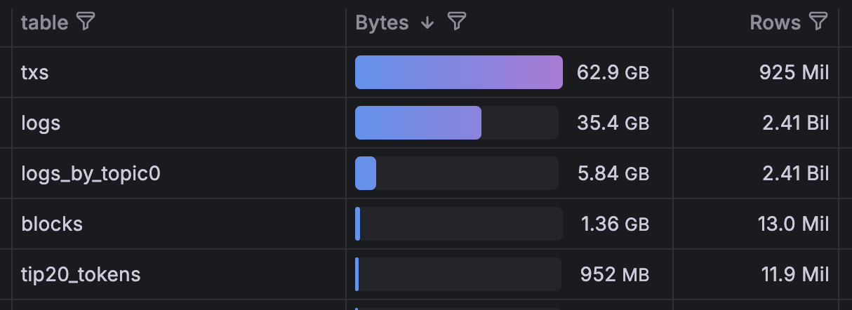
Here is the final picture of all tables after ingesting the full Tempo testnet chain and building all materialized views. The base tables (txs, logs, blocks) hold the raw chain data while logs_by_topic0 and tip20_tokens are the materialized views. Note that logs_by_topic0 covers all 2.41 billion log rows but only weighs 5.84 GB on disk (less than a sixth of the 35.4 GB base logs table) because it stores only the columns needed for address and topic lookups.
Conclusion
At this scale, ClickHouse performance is less about any single feature and more about choosing the right tradeoff for each layer of the system. On the ingestion side, batching and efficient wire formats keep write throughput high. On the storage side, choosing compression-friendly types and sort keys keeps disk usage low without sacrificing write speed. On the query side, the same sort key that is ideal for storage will not always be ideal for every access pattern, which is where materialized views become useful.
The practical lesson is that we should not try to force one table layout to serve every query equally well. A primary table such as logs can be optimized for compression and ingestion, while narrower materialized views such as logs_by_topic0 or fully decoded tables such as tip20_tokens can be optimized for specific high-value queries. That separation lets us keep the base dataset compact and flexible while still making common product and analytics queries fast enough to run interactively.